Semi-Markov Chain – I consider new job in the second year!

Napoleon’s Russian campaign
Since June 1812 to December 1812, Napoleon Bonaparte launched a large military campaign to Russia. In June, Napoleon sent his army of half a million and they occupied Moscow in September. Because of Russia’s abandon with fire, Napoleon troops had to retreat to France.
Through the retreat, it began to snow. Along with lack of food, the extreme cold weather led to great losses of lives. Among 450,000 men who entered Russia, only 120,000 men survived.
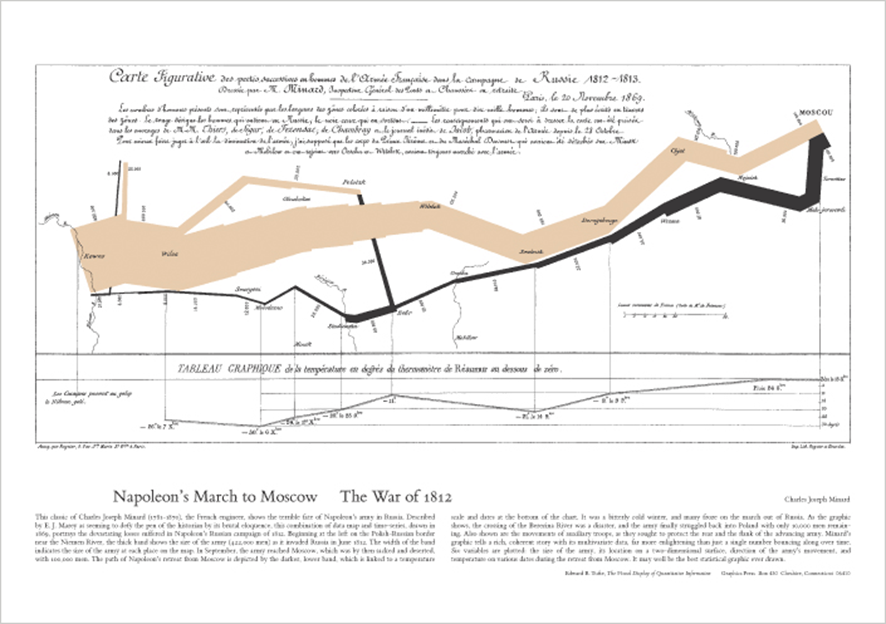
Charles Joseph Minard, a French civil engineer in 19th century, left a famous portrait of the disastrous losses by Napoleon’s Russian campaign. This portrait has been taught as a historical masterpiece of data visualization. The brown band represents number of troops from the departure to Moscow. The black narrower band represents number of troops through the retreat. The line chart in the bottom shows changing temperature during the journey. You can see gradual losses of men impacted by both time spent and cold weather.
Figure 1. Minard's portrait of Napoleon’s March

Survival Analysis
In a modern business scenario, there are needs to analyze speed of decreasing people or objects. In a medical field, rate of survivors of cancer treatment are statistically estimated through clinical trials. In an engineering, average years until machine failures are estimated from the historical data. Survival Analysis is a field of study to answer those questions.
In human resources, you want to ask ‘How many percent of the first-year employee will leave the company in two years?’ or ‘At which grade of tenure, are members most likely to promote?’
In the previous article, I walked through a modeling career transitions using Markov Chain. Though it is simple and powerful, if takes one assumption that makes difficult to apply to the real-world scenario. In this article, I will explore Semi-Markov Chain which is a refinement of the Markov Chain. To estimate accurately high-risk moment of leaving your company, it is essential to consider tenure years to model transition probability.
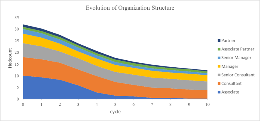
Figure 2. Example of decreasing headcount in an organization

Semi-Markov Chain
Despite the simple aspect of Markov Model, it is not realistic to apply this to a system of employee dynamics in an organization. One of the reasons is that the probability to stay, promote or quit is time-dependent by nature. It is common for an employee to stay at the same job title in the first year, but the chance of promotion becomes higher as he or she develops skills over years.
Here, another probability model called as Semi-Markov model come in. Semi-Markov Model loosens an assumption that transition probabilities are the same regardless of time spent in the grade.
Time-dependent transition probability
As an example, suppose there is an organization that consists of two job titles A and B. In the beginning, 40 people are recruited into job title A. Once a year, some of them are promoted to B. In this scenario, there are three possible transitions as follows:
(1) Staying in A
(2) Promoting to B
(3) Staying in B
Table 1. State matrix of employee transition
| Next Year | |||
| A | B | ||
| This year | A | Stay | Promotion |
| B | n/a | Stay | |
Now, let’s estimate the probability of promotion from job title A to B in three years. Table 2 illustrates step-by-step calculations for this. In the first row, I put the initial headcount (n = 40).
Next, let’s say 4 people were promoted to title B next year (t=1). This event is recorded in the second row, i.e., 4 people in column ‘A->B’ and 0.100 (4/40) in column ‘r(A, B)’.
G(A) is the survival rate. In case t = 1, G(A) =0.900, it means that 90 percent of people stay from time 0 until time 1 and this rate will be inherited to the next period t = 2 for the calculation. To calculate this, you can multiply the survival rate at the previous period t = 1 i.e., G(A)=1 with the ratio of staying people i.e., 1-r(A, B)=0.900.
The last column p(A, B) is the probability to promote from A to B. This is a multiplication of G(A) at the previous period and r(A, B) at the current period. In the second row, it is calculated as 1 * 0.100 = 0.100. In the third row, it is 0.125 which is decomposed as 0.139 * 0.900.
In the end, the cumulative probability to promote from time 0 to 3 is a summation of p(A, B) i.e., 0.375.
Table 2. Example of calculating multi-time-period transition probability
| t | n | A->B | r(A,B) | 1-r(A,B) | G(A) | p(A,B) |
| 0 | 40 | 0 | 0.000 | 1.000 | 1.000 | 0.000 |
| 1 | 40 | 4 | 0.100 | 0.900 | 0.900 | 0.100 |
| 2 | 36 | 5 | 0.139 | 0.861 | 0.775 | 0.125 |
| 3 | 31 | 6 | 0.194 | 0.806 | 0.625 | 0.150 |
| 0.375 |
What does this mean? The last column p(A, B) tells us that the third year has the highest rate of promotion 15%. Until the third year, 37.5% of people are promoted.
Conclusion
Semi-Markov chain is helpful for workforce statistics because it considers economic psychology. Employees who stay longer are not as loyal as you think. The incentive to leave your firm will be getting higher at a particular tenure. Semi-Markov model allows to estimate different transition probability over time and this will make our model be explanatory to the reality.
Reference
French invasion of Russia. (2023, January 25). In Wikipedia. https://en.wikipedia.org/w/index.php?title=French_invasion_of_Russia&oldid=1135617458
Ross, S.M. (2014). Introduction to Probability Models Eleventh Edition. Academic Press.
Tufte, E. (n.d.). POSTER: NAPOLEON’S MARCH. Retrieved January 29, 2023, from https://www.edwardtufte.com/tufte/posters